Understanding Distributed Systems Notes

I have always feel like microservice architecture is an over-engineering solution most of the times. You pay for the benefits of:

• Having clean and separated modules for different development teams
• Scalability

With the costs of:

• Building an infrastructure that support it
• The complexity of creating/debugging a distributed system.

Despite my disliking, in my interviews, the topic was brought up a lot. I tended to speak my mind and was not judged highly for that. I knew I can just practice system design interview and get by, but I wanted to get to the root of it: understanding distributed systems.

Skimming through “Understanding Distributed Systems”, I felt like it can be a good fit for me and my purpose. The book’s content is well-explained by the Preface:

Learning to build distributed systems is hard, especially if they are large scale. It’s not that there is a lack of information out there. You can find academic papers, engineering blogs, and even books on the subject. The problem is that the available information is spread out all over the place, and if you were to put it on a spectrum from theory to practice, you would find a lot of material at the two ends but not much in the middle.

That is why I decided to write a book that brings together the core theoretical and practical concepts of distributed systems so that you don’t have to spend hours connecting the dots. This book will guide you through the fundamentals of large-scale distributed systems, with just enough details and external references to dive deeper. […]

Chapter 1

Introduction

Loosely speaking, a distributed system is a group of nodes that cooperate by exchanging messages over communication links to achieve some task.

Why do we bother building distributed systems in the first place?

• […] some applications require high availability and need to be resilent to single-node failures. […]
• Some applications need to tackle workloads that are just too big to fit on a single node, no matter how powerful. […]
• […], some applications have performance requirements that would be physically impossible to achieve with a single node. […]

This book tackles the fundamental challenges that needed to be solved to: design, build, and operate distributed systems.

Basically, a distributed system is a network of nodes that communicate with each other. They replace single nodes to avoid single-node failures, handle big workloads (data and computation?), and have good performance (latency?).

1.1 Communication

The first challenge derives from the need for nodes to communicate with each other over the network. […]

Although it would be convenient to assume that some networking library is going to abstract all communication concerns away, in practice, it’s not that simple because abstractions leak, and you need to understand how the network stack works when that happens.

I would leave a note of a story that I heard from an interviewer on profiling, and try to link everything together later. He investigated on why is the company’s microservice is not having a good latency: there are some input services that fetch data from 3rd parties. The bottleneck lies at the way JSON is deserialized from those services.

1.2 Coordination

Another hard challenge of building distributed systems is that some form of coordination is required to make individual nodes work in unison towards a shared objective. This is particularly challenging to do in the presence of failures. […]

1.3 Scalability

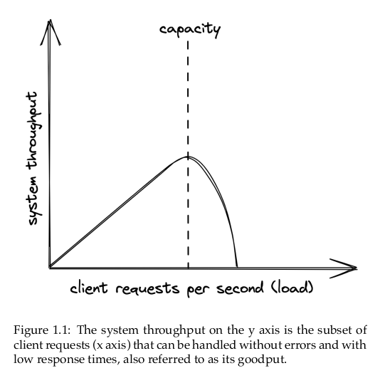
The performance of an application represents how efficiently it can handle load. Intuitively, load is anything that consumes the system’s resources such as CPU, memory, and network bandwidth. Since the nature of load depends on the application’s use cases and architecture, there are different ways to measure it. […]

For the type of applications discussed in this book, performance is generally measured in terms of throughput and response time. Throughput is the number of requests processed per second by the application, while response time is the time elapsed in seconds between sendinga request to the application and receiving a response.

As load increases, the application will eventually reach its capacity, i.e., the maximum load it can withstand, when a resource is exhauted. The performance either plateaus or worsens at that point, […]. If the load on the system continues to grow, it will eventually hit a point where most operations fail or time out.

The capacity of a distributed system depends on:

• Its architecture,
• Its implementation,
• And an intricate web of physical limitations like the nodes’ memory size and clock size and clock cycle and the bandwidth and latency of network links.

For an application to be scalable, a load increase should not degrade the application’s performance, This requires increasing the capacity of the application at will.

A quick an easy way is to buy more expensive hardware with better performance, which is also referred to as scaling up. Unfortunately, this approach is bound to hit a brick wall sooner or later when such hardware just doesn’t exist. The alternative is scaling out by adding more commodity machines to the system and having them work together.

Another word for scaling up is scaling vertically, and for scaling out is scaling horizontally.

1.4 Resiliency

A distributed system is resilient when it can continue to do its job even when failures happen. And at scale, anything that can go wrong will go wrong. Every component has a probability of failing – nodes can crash, network links can be severed, etc. […]

Failures that are left unchecked can impact the system’s availability, i.e., the percentage of time the system is available to use. It’s a ratio defined as the amount of time the application can serve requests (uptime) divided by the total time measured (uptime plus downtime, i.e., the time the application can’t serve requests).

[…]

If the system isn’t resilient to failures, its availability will inevitably drop. Because of that, a distributed system needs to embrace failures and be prepared to withstand them using techniques such as:

• Redundancy
• Fault isolation
• Self-healing mechanisms

[…]

1.5 Maintainability

Any change is a potential incident waiting to happen. Good testing – in the form of unit, integration, and end-to-end tests – is a minimum requirement to modify or extend a system without worrying it will break. And once a change has been merged into the codebase, it needs to be released to production safely without affecting the system’s availability.

Also, operators operators need to:

• Monitor the system’s health,
• Investigate degradations, and
• Restore the service when it can’t self-heal.

This requires altering the system’s behavior without code changes, e.g., toggling a feature flag or scaling out a service with a configuration change.

1.6 Anatomy of a distributed system

[…] In this book, we are mainly concerned with backend applications that run on commodity machines and implement some kind of business service. So you could say a distributed system is a group of machines that communicate over network links. However, from a run-time point of view, a distributed system is a group of software processes that communicate via inter-process communication (IPC) mechanisms like HTTP. And from an implementation point perspective, a distributed system is a group of loosely-coupled components (services) that communicate via APIs.

Some Thoughts

The author walked the readers (at least me) gently through distributed systems in this chapter. I like the way he tried to minimize the jargons (or that the jargons can be well-understood for his intended readers).

I hoped that at the end of the book, I would be able to consolidate something like a “first principle” about distributed systems, like I did after reading SICP. Implemented an interpreter on my own, I had taken by heart the term “homoiconicity”: code is data. A program works by having another program that reads the first program’s text and executes it.

Part 1 Communication

Introduction

Communication between processes over the network, or interprocess communication (IPC), is at the heart of distributed systems – it’s what make distributed systems distributed. In order for processes to communicate, they need to agree on a set of rules that determine how data is processed and formatted. Network protocols specify such rules.

The protocols are arranged in a stack, where each layer builds on the abstraction provided by the layer below, and lower layers are closer to the hardware. When a process sends data to another through the network stack, the data moves from the top layer to the bottom layer and vice-versa at the other end […].

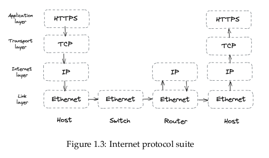
I found another good explanation diagram from the Internet, and will just put it here for later revision.

Chapter 2 Reliable links

At the internet layer, the communication between two nodes happens by routing packets to their destination from one router to the next. Two ingredients are required for this: a way to address nodes and a mechanism to route packets across routers.

Addressing is handled by the IP protocol. For example, IPv6 provides a 128-bit address space, allowing 2^128 addresses. To decide where to send a packet, a router needs to consult a local routing table. The table maps a destination address to the address of the next router along the path to that destination. The responsibility of building and communicating the routing tables across routers lies with the Border Gateway Protocol (BGP).

The author also linked to RFC 4271: https://datatracker.ietf.org/doc/html/rfc4271. At the moment, I felt that BGP is a nice-to-have knowledge, but is not something too crucial.

Now, IP doesn’t guarantee that data sent over the internet will arrive at its destination. For example, if a router becomes over-loaded, it might start dropping packets. This is where TCP comes in, a transport-layer protocol that exposes a reliable communication channel between two processes on top of IP. TCP guarantees that a stream of bytes arrives in order without gaps, duplication, or corruption. TCP also implements a set of stability patterns to avoid overwhelming the network and the receiver.

Previously, the author linked to The Law of Leaky Abstraction when he mentioned “leaking abstraction”. The article has a really cool analogy of how TCP is built:

Imagine that we had a way of sending actors from Broadway to Hollywood that involved putting them in cars and driving them across the country.

• Some of these cars crashed, killing the poor actors.
• Sometimes the actors got drunk on the way and shaved their heads or got nasal tattoos, thus becoming too ugly to work in Hollywood, and
• Frequently the actors arrived in a different order than they had set out, because they all took different routes.

Now imagine a new service called Hollywood Express, which delivered actors to Hollywood, guaranteeing that they would (a) arrive (b) in order (c) in perfect condition. The magic part is that Hollywood Express doesn’t have any method of delivering the actors, other than the unreliable method of putting them in cars and driving them across the country.

Hollywood Express works by checking that each actor arrives in perfect condition, and, if he doesn’t, calling up the home office and requesting that the actor’s identical twin be sent instead.

• If the actors arrive in the wrong order Hollywood Express rearranges them.
• If a large UFO on its way to Area 51 crashes on the highway in Nevada, rendering it impassable, all the actors that went that way are rerouted via Arizona and Hollywood Express doesn’t even tell the movie directors in California what happened.

To them, it just looks like the actors are arriving a little bit more slowly than usual, and they never even hear about the UFO crash.

That is, approximately, the magic of TCP. It is what computer scientists like to call an abstraction: a simplification of something much more complicated that is going on under the covers.

2.1 Reliability

To create the illusion of a reliable channel, TCP partitions a byte stream into discrete packets called segments. The segments are sequentially numbered, which allows the receiver to detect holes and duplicates. Every segment needs to be acknowledged by the receiver. When that doesn’t happen, a timer fires on the sending side and the segment is retransmitted. To ensure that the data hasn’t been corrupted in transit, the receiver uses a checksum to verify the integrity of a delivered segment.

2.2 Connection lifecycle

A connection needs to be opened before any data can be transmitted on a TCP channel. The operating system manages the connection state on both ends through a socket.

I was intrigued by the word socket on encountering it many times before, but could not fully explain what it is. I guessed I have to borrow this definition, and go with it for now:

A network socket is a software structure within a network node of a computer network that serves as an endpoint for sending and receiving data across the network.

https://en.wikipedia.org/wiki/Network_socket

Windows has Winsock, while Unix/Linux has Unix Domain Socket, which is a file.

The socket keeps track of the state changes of the connection during its lifetime. At a high level, there are three states the connection could be in:

• The opening state in which the connection is being created.
• The established state in which the connection is open and data is being transferred.
• The closing state in which the connection is being closed.

In reality, this is a simplification, as there are more states than the three above.

A server must be listening for connection requests from clients before a connection is established. TCP uses a three-way handshake to create a new connection, as shown in Figure 2.1:

1. The sender picks a random sequence number x and sends a SYN segment to the receiver
2. The receiver increments x, chooses a random sequence number y, and sends back a SYN/ACK segment
3. The sender increments both sequence numbers and replies with an ACK segment and the first bytes of application data.

I found the author’s diagram is kind of hard to understand with the original font, so I created one my own:

The handshake introduces a full round-trip in which no application data is sent. So until the connection has been opened, the bandwidth is essentially zero.

I found this really confusing and contradicted to the author’s earlier statement: “The sender increments both sequence numbers and replies with an ACK segment the first bytes of application data”.

The lower the round trip time is, the faster the connection can be established. Therefore, putting servers close to the clients helps reduce this cold-start penalty.

After the data transmission is complete, the connection needs to be closed to release all resources on both ends. This termination phase involves multiple round-trips. If it’s likely that another transmission will occur soon, it makes sense to keep the connection open to avoid paying the cold-start tax again.

Moreover, closing a socket doesn’t dispose of it immediately as it transitions to a waiting state (TIME_WAIT) that lasts several minutes and discards any segments received during the wait. The wait prevents delayed segments from a closed connection from being considered a part of a new connection. But if many connections open and close quickly, the number of sockets in the waiting state will continue to increase until it reaches the maximum number of sockets that can be open, causing new connection attempts to fail. This is another reason why processes typically maintain connection pools to avoid recreating connections repeatedly.

I thought these are good bits of wisdom. It is related to a database’s connection pool, but I would keep it at that and try to have a deeper understanding later.

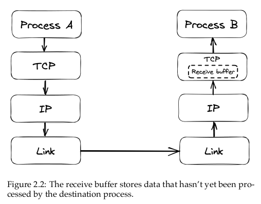
2.3 Flow control

Flow control is a backoff mechanism that TCP implements to prevent the sender from overwhelming the receiver. The receiver stores incoming TCP segments waiting to be processed by the application into a receive buffer […].

The receiver also communicates the size of the buffer to the sender whenever it acknowledges a segment […]. Assuming it’s respecting the protocol, the sender avoids sending more data that can fit in the receiver’s buffer.

[…]

This mechanism is not too dissimilar to rate-limiting at the service level, a mechanism that rejects a request when a specific quota is exceeded […]. But, rather than rate-limiting on an API key or IP address, TCP is rate-limiting on a connection level.

2.4 Congestion control

TCP guards not only agains overwhelming the receiver, but also against flooding the underlying network. The sender maintains a so-called congestion window, which represents the total number of outstanding segments that can be sent without an acknowledgement from the other side. The smaller the congestion window is, the fewer bytes can be in flight at any given time, and the less bandwidth is utilized.

When a new connection is established, the size of the congestion window is set to a system default. Then, for every segment acknowledged, the window increases its size exponentially until it reaches an upper limit. This means we can’t use the network’s full capacity right after a connection is established. The shorter the round-trip time (RTT), the quicker the sender can start utilizing the underlying network’s bandwidth […].

What happens if a segment is lost? When the sender detects a missed acknowledgement through a timeout, a mechanism called congestion avoidance kicks in, and the congestion window size is reduced. From there onwards, the passing of time increases the window size by a certain amount, and timeouts decrease it by another.

[…], we can derive the maximum theoretical bandwidth by dividing the size of the congestion window by the round trip time:

bandwidth = winSize / RTT

The equation shows that bandwidth is a function of latency. TCP will try very hard to optimize the window size since it can’t do anything about the round-trip time. However, that doesn’t always yield the optimal configuration. Due to the way congestion control works, the shorter the round-trip time, the better the underlying network’s bandwidth is utilized. This is more reason to put servers geographically close to the clients.

2.5 Custom protocols

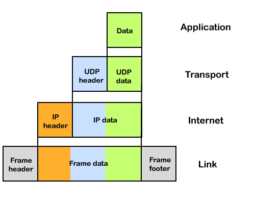
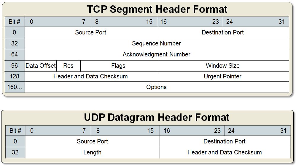
TCP’s reliability and stability come at the price of lower bandwidth and higher latencies than the underlying network can deliver. If we drop the stability and reliability mechanisms that TCP provides, what we get is a simple protocol named User Diagram Protocol (UDP) – a connectionless transport layer protocol that can be used as an alternative to TCP.

Unlike TCP, UDP does not expose the abstraction of a byte stream to its clients. As a result, clients can only send dicrete packets with a limited size called datagrams. UDP doesn’t offer any reliability as datagrams don’t have sequence numbers and are not acknowledged. UDP doesn’t implement flow and congestion control either. Overall, UDP is a lean and bare-bones protocol. It’s used to bootstrap custom protocols, which provide some, but not all, of the stability and reliability guarantees that TCP does.

I think adding a diagram to compare the two protocols’ headers can also be helpful here:

For example, in multiplayer games, clients sample gamepad events several times per second and send them to a server that keeps track of the global game state. Similarly, the server samples the game state several times per second and sends these snapshots back to the clients. If a snapshot is lost in transmission, there is no value in retransmitting it as the game evolves in real-time; by the time the retransmitted snapshot would get to the destination, it would be obsolete. This is a use case where UDP shines; in contrast, TCP would attempt to redeliver the missing data and degrade the game’s experience.

The example is on point here. Real-time video streaming can also be a good sample case.

Some Thoughts

I tried to implementing a “barebone” TCP, where a sender and a receiver is exchanging messages via channels. The method of using an ACK works. Simulating network congestion needs more time and thought, so I would revisit it later.

Chapter 3 Secure links

I felt like this chapter is another nice-to-have piece of knowledge, so I would revisit it at another time.

Chapter 4 Discovery

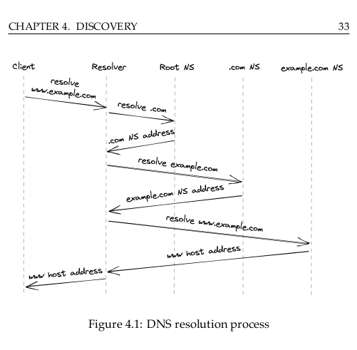
[…], we have explored how to create a reliable and secure channel between two processes running on different machines. However, to create a new connection with a remote process, we must first discover its IP address somehow. The most common way of doing that is via the phone book of the internet: the Domain Name System (DNS) – a distributed, hierarchical, and eventually consistent key-value store.

In this chapter, we will look at how DNS resolution works in a browser, but the process is similar to other types of clients. When you enter a URL in your browser, the first step is to resolve the hostname’s IP address, which is then used to open a new TLS connection. […]

Chapter 5 APIs

The communication style between a client and a server can be direct or indirect, depending on whether the client communicates directly with the server or indirectly through a broker.

Direct communication requires that both processes are up and running for the communication to be succeed. However, sometimes this guarantee is either not needed or very hard to achieve, in which case indirect communication is a better fit.

An example of indirect communication is messaging. In this model, the sender and the receiver don’t communicate directly, but they exchange messages through a message channel (the broker). The sender sends messages to the channel, and on the other side, the receiver reads messages from it. […]

In this chapter, we will focus our attention on a direct communication style called request-response, in which a client sends a request message to the server, and the server replies with a response message. This is similar to a function call but across process boundaries and over the network.

The request and response messages contain data that is serialized in a language-agnostic format. The choice of format determines a message’s serialization and deserialization speed, whether it’s human-readable, and how hard it is to evolve over time. A textual format like JSON is self-describing and human-readable, at the expense of increased verbosity and parsing overhead. On the other hand, a binary format like Protocol Buffers is leaner and more perfomant than a textual one at the expense of human readability.

When a client sends a request to a server, it can block and wait for the response to arrive, making the communication synchronous. Alternatively, it can ask the outbound adapter to invoke a callback when it receives the response, making the communication asynchronous.

Synchronous communication is inefficient, as it blocks threads that could be used to do something else. Some languages, like JavaScript, C#, and Go, can completely hide callbacks through language primitives such as async/await. These primitives make writing asynchronous code as straightforward as writing synchronous code.

Commonly used IPC technology for request-response interactions are HTTP and gRPC. Typically, internal APIs used for server-to-server communications within an organization are implemented with a high-performance RPC framework like gRPC. In contrast, external APIs is available to the public tend to be based on HTTP, since web browsers can easily make HTTP requests via JavaScript code.

A popular set of design principles for designing elegant and scalable HTTP APIs is representational state transfer (REST), and an API based on these principles is said to be RESTful. For example, these principles include that:

• requests are stateless, and therefore each request contains all the necessary information required to process it;
• responses are implicitly or explicitly labeled as cachable or non-cachable. If a response is cachable, the client can reuse the response for a later, equivalent request.

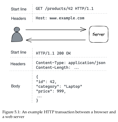
5.1 HTTP

HTTP is a request-response protocol used to encode and transport information between a client and a server. In an HTTP transaction, the client sends a request message to the server’s API endpoint, and the server replies back with a response message […].

[…]

HTTP 1.1 keeps a connection to a server open by default to avoid needing to create a new one for the next transaction. However, a new request can’t be issued until the response to the previous one has been received (aka head-of-line blocking or HOL blocking); in other words, the transactions have to be serialized. For example, a browser that needs to fetch several images to render an HTML page has to download them one at a time, which can be very inefficient.

Although HTTP 1.1 technically allows some type of requests to be pipelined, it still suffers from HOL blocking as a single slow response will block all the responses after it. With HTTP 1.1, the typical way to improve the throughput of outgoing requests is by creating multiple connections. However, this comes with a price because connections consume resources like memory and sockets.

HTTP 2 was designed from the ground up to address the main limitations of HTTP 1.1. It uses a binary protocol rather than a textual one, allowing it to multiplex multiple concurrent request-response transactions (streams) on the same connection. In early 2020 about half of the most-visited websites on the internet were using the new HTTP 2 standard.

HTTP 3 is the latest iteration of the HTTP standard, which is based on UDP and implements its own transport protocol to address some of TCP’s shortcomings. For example, with HTTP 2, a packet loss over the TCP connection blocks all streams (HOL), but with a HTTP 3 a packet loss interrupts only one stream, not all of them.

5.2 Resources

5.3 Request methods

5.4 Response status codes

5.5 OpenAPI

5.6 Evolution

5.7 Idempotency

Some Notes

I skipped section 5.2 to 5.7 since they do have some useful information on writing APIs, but they are not my main focus on reading the book.

Part II Coordination

Introduction

[…] Our ultimate goal is to build a distributed application made of a group of processes that gives its users the illusion that they are interacting with on coherent node. Although achieveing a perfect illusion is not always that possible or desirable, some degree of coordination is always needed to build a distributed application.

In this part, we will explore the core distributed algorithms at the heart of distributed applications. […]

Chapter 6 System models

To reason about distributed systems, we need to define precisely what can and can’t happen. A system model encodes expectations about the behavior of

• Processes
• Communication links
• Timing

Think of it as a set of assumptions that allow us to reason about distributed systems by ignoring the complexity of the actual technologies used to implement them.

For example, these are some common models for communication links:

• The fair-loss link model assumes that messages may be lost and duplicated, but if the sender keeps retransmitting a message, eventually it will be delivered to the destination.
• The reliable link model assumes that a message is delivered exactly once, without loss or duplication. A reliable link can be implemented on top of a fair-loss one by de-duplicating messages at the receiving side.
• The authenticated reliable link model makes the same assumptions as the reliable link but additionally assumes that the receiver can authenticate the sender.

[…], we can model the behavior of processes based on the type of failures we expect to happen:

• The arbitrary-fault model assumes that a process can deviate from its algorithm in arbitrary ways, leading to crashes or unexpected behaviors caused by bugs or malicious activity. For historical reasons, this model is also referred to as the “Byzantine” model. More interestingly, it can be theoretically proven that a system using this model can tolerate up to 1/3 of faulty processes and still operate correctly.
• The crash-recovery model assume that a process doesn’t deviate from its algorithm but can crash and restart at any time, losing its in-memory state.
• The crash-stop model assumes that a process doesn’t deviate from its algorithm but doesn’t come back online if it crashes. Although this seems unrealistic for software crashses, it models the unrecoverable hardware faults and generally makes the algorithms simpler.

The arbitrary-fault model is typically used to model safety-critical systems like airplane engines, nuclear power plants, and systems where a single entity doesn’t fully control all the processes (e.g., digital cryptocurrencies such as Bitcoin). These use cases are outside the book’s scope, and the algorithms presented here will generally assume a crash-recovery model.

Finally, we can also model timing assumptions:

• The synchronous model assumes that sending a message or executing an operation never takes more than a certain amount of time. This is not very realistic for the type of systems we care about, where we know that sending messages over the network can potentially take a very long time, and processes can be slowed down by, e.g., garbage collection cycles or page faults.
• The asynchronous model assumes that sending a message or executing an operation on a process can take an unbounded amount of time. Unforunately, many problems can’t be solved under this assumption; if sending messages can take an infinite amount of time, algorithms can get stuck and not make any progress at all. Nevertheless, this model is useful because it’s simpler than models that make timing assumptions, and therefore algorithms based on it are also easier to implement.
• The partially synchronous model assumes that the system behaves synchronously most of the time. This model is typically representative enough of real-world systems.

In the rest of the book, we will generally assume a system model with fair-loss links, crash-recovery processes, and partial synchrony. […]

But remember, models are just an abstraction of reality since they don’t represent the real world with all its nuances. So, as you read along, question the models’ assumptions and try to imagine how algorithms that rely on them could break in practice.

I found this chapter really useful, and can be used as a part of a more general framework on thinking about distributed systems. In short, we can divide a distributed system into three parts:

• Processes
• Communication
• Timing

On each part, we can have some “levels” of assumption, depends on the rigour of the system. For example, with something as mission-critical as a plane’s flight system, we must be more careful.

With processes, there are:

• The arbitrary-fault model: everything can go wrong and unexpected behaviors are to be expected
• The crash-recovery model: there can be crashes and restarts
• The crash-stop model: once it crashes, it does not come back

With communication, there are:

• The fair-loss link model: messages may be lost and duplicated, but will eventually reach the destination with enough retry
• The reliable link model: messages are delivered exactly once, without loss and duplication
• The authenticated reliable link model: the same as above, but with authentication

With timing, there are:

• The synchronous model: operations are guaranteed to be success in a fixed amount of time
• The asynchronous model: operations can take forever
• The partially synchronous model: operations succeed most of the times

Chapter 7 Failure detection

A ping is a periodic request that a process sends to another to check whether it’s still available. The process expects a response to the ping within a specific time frame. If no response is received, a timeout triggers and the destination is considered unavailable. However, the process will continue to send pings to it to detect if and when it comes back online.

A heartbeat is a message that a process periodically sends to another. If the destination doesn’t receive a heartbeat wihtin a specific time frame, it triggers a timeout and considers the process unavailable. But if the process comes back to life later and starts sending out heartbeats, it will eventually be considered to be available again.

Pings and heartbeats are generally used for processes that interact with each other frequently, in situations where an action needs to be taken as soon as one of them is no longer reachable. In other circumstances, detecting failures just at communication time is good enough.

Chapter 8 Time

Time is an essential concept in any software application; even more so in distributed ones. We have seen it play a crucial role in the network stack (e.g., DNS record TTL) and failure detection (timeouts). Another important use of it is for ordering events.

[…] in a distributed system, there is no shared global clock that all processes agree on that can be used to order operations. And, to make matter worse, processes can run concurrently.

It’s challenging to build distributed applications that work as intended without knowing whether one operation happened before another. In this chapter, we will learn about a family of clocks that can be used to work out the order of operations across processes in a distributed system.

8.1 Physical clocks

[…] most operating systems offer a different type of clock that is not affected by time jumps: a monotonic clock. A monotonic clock measures the number of seconds elapsed since an arbitrary point in time (e.g., boot time) and can only move forward. A monotonic clock is useful for measuring how much time has elapsed between two timestamps on the same node. However, monotonic clocks are of no use for comparing timestamps of different nodes.

Since we don’t have a way to synchronize wall-time clocks across processes perfectly, we can’t depend on them for ordering operations across nodes. To solve this problem, we need to look at it from another angle. We know that two operations can’t run concurrently in a single-threaded process as one must happen before the other. This happened-before relationship creates a causal bond between the two operations, since the one that happens first can have side-effects that affect the operation that comes after it. We can use this intuition to build a different type of clock that isn’t tied to the physical concept of time but reather captures the causal relationship between operations: a logical clock.

8.2 Logical clocks

A logical clock measures the passing of time in terms of logical operations, not wall-clock time. The simplest possible logical clock is a counter, incremented before an operation is executed. Doing so ensure that each operation has a distinct logical timestamp. If two operations execute on the same process, then necessarily one must come before the other, and their logical timestamps will reflect that. But what about operations executed on different processes?

[…] Similarly, when one process sends a message to another, a so-called synchronization point is created. The operations executed by the sender before the message was sent must have happened before the operations that the receiver executed after receiving it.

A Lamport clock is a logical clock based on this idea. To implement it, each process in the system needs to have a local counter that follows specific rules:

• The counter is initialized with 0.
• The process increments its counter by 1 before executing an operation.
• When the process sends a message, it increments its counter by 1 and sends a copy of it in the mssage.
• When the process receives a message, it merges the counter it received with its local counter by taking the maximum of the two. Finally, it increments the counter by 1.

I find the idea interesting and can understand the idea behind, but is not too sure where can I apply it.

8.3 Vector clocks

A vector clock is a logical clock that guarantees that if a logical timestamp is less than another, then the former must have happened before the latter. A vector clock is implemented with an array of counters, one for each process in the system. And, as with Lamport clocks, each process has its own copy.

Basically, instead of having a single number, vector clocks have a vector of timestamps.

This discussion about logical clocks might feel a bit abstract at this point but bear with me. Later in the book, we will encounter some practical applications of logical clocks. What’s important to internalize at this point is that, in general, we can’t use physical clocks to accurately derive the order of events that happened on different processes. That being said, sometimes physical clocks are good enough. For example, using physical clocks to timestamp logs may be fine if they are only used for debugging purposes.

Chapter 9 Leader election

There are times when a single process in the system needs to have special powers, like accessing a shared resource or assigning work to others. To grant a process these powers, the system needs to elect a leader among a set of candidate processes, which remains in charge until it relinquishes its role or becomes otherwise unavailable. When that happens, the remaining processes can elect a new leader among themselves.

A leader election algorithm needs to guarantee that there is at most one leader at any given time and that an election eventually completes even in the presence of failures. These two properties are also referred to as safety and liveness, respectively, and they are general properties of distributed algorithms. Informally, safety guarantees that nothing bad happens and liveness that something good eventually does happen. […]

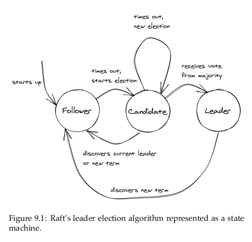
9.1 Raft leader election

Raft’s leader election algorithm is implemented as a state machine in which any process is in one of three states (see Figure 9.1):

• the follower state, where the process recognizes another one as the leader;
• the candidate state, where the process starts a new election proposing itself as a leader;
• or the leader state, where the process is the leader.

In Raft, time is divided into election terms of arbitrary length that are numbered with consecutive integers (i.e., logical timestamps). A term begins with a new election, during which one or more candidates attempt to become the leader. The algorithm guarantees that there is at most one leader for any term. But what triggers an election in the first place?

When the system starts up, all processes begin their journey as followers. A follower expects to receive a periodic heartbeat from the leader containing the election term the leader was elected in. If the follower doesn’t receive a heartbeat within a certain period of time, a timeout fires and the leader is presumed dead. At that point, the follower starts a new election by incrementing the current term and transitioning to the candidate state. It then votes for itself and sends a request to all the processes in the system to vote for it, stamping the request with the current election term.

The process remains in the candidate state until one of three things happens: it wins the election, another process wins the election, or some time goes by with no winner:

• The candidate wins the election – The candidate wins the election if the majority of processes in the system vote for it. Each process can vote for at most one candidate in a term on a first-come-first-served basis. This majority rule enforces that at most one candidate can win a term. If the candidate wins the election, it transitions to the leader state and starts sending heartbeats to the other processes.
• Another process wins the election – If the candidate receives a heartbeat from a process that claims to be the leader with a term greater than or equal to the candidate’s term, it accepts the new leader and returns to the follower state. If not, it continues in the candidate state. You might be wondering how that could happen; for example, if the candidate process was to stop for any reason, like for a long garbage collection pause, by the time it resumes another process could have won the election.
• A period of time goes by with no winner – It’s unlikely but possible that multiple followers become candidates simultaneously, and none manages to receive a majority of votes; this is referred to as a split vote. The candidate will eventually time out and start a new election when that happens. The election timeout is picked randomly from a fixed interval to reduce the likelihood of another split vote in the next election.

Researching on Raft led me to Paxos, which is an older distributed algorithm. I feel like there are some similarities between the Raft leader election algorithm and the single-decree Paxos described by Martin Fowler in his article.

There is this picture that explains Raft states that belongs to the next section, but including it here seems to be more appropriate. The original source is from Raft’s paper itself that the author linked.

Tried to implement a Raft leader election simulation for learning purpose, I will try to put Raft’s ideas to a more coherent form for implementation:

Suppose we have a system that consists of processes (the processes are computation units that have their own states and can send messages to themselves or to other processes)

Each process can be in one of three states:

• The follower state: the process recognizes another process as the leader
• The candidate state: the process tries to elect itself (or another process) as the leader
• The leader state: the process is the leader, and it sends heartbeats to other processes

At the beginning, all processes are followers.

A process changes its state following the state diagram above, or:

• Follower -> Candidate: if it does not receive a heartbeat after a fixed time
• Candidate -> Leader: its vote count is the highest
• Any -> Follower: it receive a “new” heartbeat

How do we know if a heartbeat is “new”? The answer is that each process has a logical timestamp called “election term”. The processes will comply to “newer messages” (or messages that have greater election term).

Here are the message types:

• Timeout: a follower sends this to itself to change its state to candidate
• Hearbeat: the leader sends this to other followers
• Vote Request: a candidate sends this to other processes
• Promotion: a candidate sends this to itself after it received enough vote

We see the Cartesian product of the message types and the process types to see how should we handle each case:

9.2 Practical considerations

There are other leader election algorithms out there, but Raft’s implementation is simmple to understand and also widely used in practice […]. In practice, you will rarely, if ever, need to implement leader election from scratch. A good reason for doing that would be if you needed a solution with zero external dependencies. Instead, you can use any fault-tolerant key-value store that offers a linearizable compare-and-swap operation with an expiration time (TTL).

The author went on various considerations of using compare-and-swap that is nice-to-know, but I did not think that I needed it right then.

Although having a leader can simplify the design of a system as it eliminates concurrency, it can also become a scalability bottleneck if the number of operations performed by it increases to the point where it can no longer keep up. Also, a leader is a single point of failure with a large blast radius; if the election process stops working or the leader isn’t working as expected, it can bring down the entire system with it. We can mitigate some of these downsides by introducing partitions and assigning a different leader per partition, but that comes with additional complexity. This is the solution many distributed data stores use since they need to use partitioning anyway to store data that doesn’t fit in a single node.

As a rule of thumb, if we must have a leader, we have to minimize the work it perfoms and be prepared to occasionally have more than one.

Taking a step back, a crucial assumption we made earlier is that the data store that holds leases is fault-tolerant, i.e., it can tolerate the loss of a node. Otherwise, if the data store ran on a single node and that node were to fail, we wouldn’t be able to acquire leases. For the data store to withstand a node failing, it needs to replicate its state over multiple nodes. […]

Chapter 10 Replication

Data replication is a fundamental building block of distributed systems. One reason for replicating data is to increase availability. If some data is stored exclusively on a single process, and that process goes down, the data won’t be accessible anymore. However, if the data is replicated, clients can seemlessly switch to a copy. Another reason for replication is to increase scalability and performance; the more replicas there are, the more clients can access the data concurrently.

Implementing replication is challenging because it requires keeping replicas consistent with one another even in the face of failures. In this chapter, we will explore Raft’s replication algorithm, a replication protocol that provides the strongest consistency guarantee possible – the guarantee that to clients, the data appears to be stored on a single process, even if it’s acutally replicated. […]

Raft is based on a mechanism known as state machine replication. The main idea is that a single process, the leader, broadcasts operations that change its state to other processes, the followers (or replicas). If the followers execute the same sequence of operations as the leader, then each follower will end up in the same state as the leader. Unfortunately, the leader can’t simply broadcast operations to the followers and call it a day, as any process can fail at any time, and the network can lose messages. This is why a large part of the algorithm is dedicated to fault tolerance.

The reason why this mechanism is called state machine replication is that each process is modeled as a state machine that transitions from one state to another in response to some input (an operation). If the state machines are deterministic and get exactly the same input in the same order, their states are consistent. That way, if one of them fails, a redundant copy is available from any of the other state machines. State machine replication is a very powerful tool to make a service fault-tolerant as long as it can be modeled as a state machine.

There is a minor typo in this page: the author wrote “this this mechanism is called stated machine”.

10.1 State machine replication

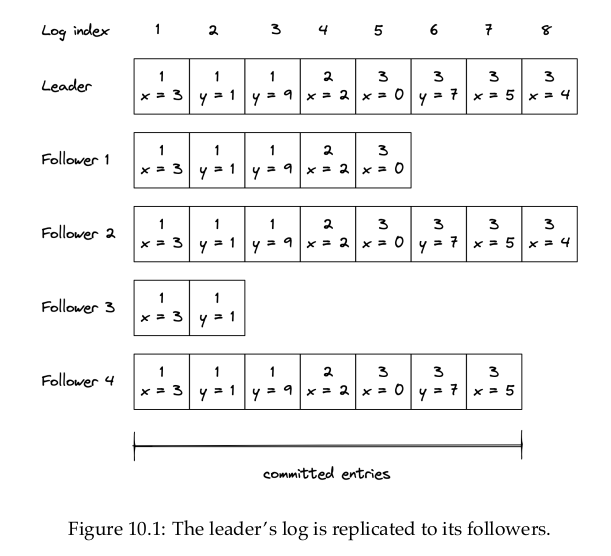
When the system starts up, a leader is elected using Raft’s leader election algorithm discussed in chapter 9, which doesn’t require any external dependencies. The leader is the only process that can change the replicated state. It does so by storing the sequence of operations that alter the state into a local log, which it replicates to the followers. Replicating the log is what allows the state to be kept in sync across processes.

[…], a log is an ordered list of entries where each entry includes:

• the operation to be applied to the state, […]. The operation needs to be deterministic so that all followers end up in the same state, but it can be arbitrarily compex as long as the requirement is respected (e.g., compare-and-swap or a transaction with multiple operations);
• the index of the entry’s position in the log;
• and the leader’s election term (the number in each box).

When the leader wants to apply and operation to its local state, it first appends a new entry for the operation to its log. At this point, the operation hasn’t been applied to the local state just yet; it has only been logged.

The leader then sends an AppendEntries request to each follower with the new entry to be added. This message is also sent out periodically, even in the absence of new entries, as it acts as a heartbeat for the leader.

When a follower receives an AppendEntries request, it appends the entry it received to its own log (without actually executing the operation yet) and sends back a response to the leader to acknowledge that the request was successful. When the leader hears back successfully from a majority of followers, it considers the entry to be committed and executes the operation on its local state. The leader keeps track of the highest committed index in the log, which is sent in all future AppendEntries requests. A follower only applies a log entry to its local state when it finds out that the leader has committed the entry.

Because the leader needs to wait for only a majority (quorum) of followers, it can make progress even if some are down, i.e., if there are 2f + 1 followers, the system can tolerate up to f failures. The algorithm guarantees that an entry that is committed is durable and will eventually be executed by all the processes in the system, not just those that were part of the original majority.

So far, we have assumed there are no failures, and the network is reliable. Let’s relax those assumptions. If the leader fails, a follower is elected as the new leader. But, there is a caveat: because the replication algorithm only needs a majority of processes to make progress, it’s possible that some processes are not up to date when a leader fails. To avoid an out-of-date process becoming the leader, a process can’t vote for one with a less up-to-date log. In other words, a process can’t win an election if it doesn’t contain all committed entries.

To determine which of two processes’ logs is more up-to-date, the election term and index of their last entries are compared. If the logs end with different terms, the log with the higher terms is more up to date. If the logs end with the same term, whichever log is longer is more up to date. Since the election requires a majority vote, and a candidate’s log must be at least as up to date as any other process in that majority to win the election, the elected process will contain all committed entries.

If an AppendEntries request can’t be delivered to one or more followers, the leader will retry sending it indefinitely until a majority of the followers have successfully appended it to their logs. Retries are harmless as AppendEntries requests are idempotent, and follower ignore log entries that have already been appended to their logs.

If a follower that was temporarily unavailable comes back online, it will eventually receive an AppendEntries message with a log entry from the leader. The AppendEntries message includes the index and term number of the entry in the log that immediately precedes the one to be appended. If the follower can’t find a log entry with that index and term number, it rejects the message to prevent creating a gap in its log.

When the AppendEntries request is rejected, the leader retries the request, this time including the last two log entries – this is why we referred to the request as AppendEntries and not as AppendEntry. If that fails, the leader retries sending the last three log entries and so forth. The goal is for the leader to find the latest log entry where the two logs agree, delete any entries in the follower’s log after that point, and append to the follower’s log all of the leader’s entries after it.

10.2 Consensus

By solving state machine replication, we actually found a solution to consensus – a fundamental problem studied in distributed systems research in which a group of processes has to decide a value so that:

• every non-faulty process eventually agrees on a value;
• the final decision of every non-faulty process is the same everywhere;
• and the final value that has been agreed on has been proposed by a process.

[…] Another way to think about consensus is the API of a write-once register (WOR): a thread-safe and linearizable register that can only be written once but can be read many times.

I thought this is the second time the author mentions the word “linearizable”. I got curious about it and read ahead. So “linearizability” is related to “consistency models”, and it is the strongest form of consistency. Another source explains it as “all operations are executed in a way as if executed on a single machine, despite the data being distributed across multiple replicas. As a result, every operation returns an up-to-date value.”

There are plenty of practical applications of consensus. For example, agreeing on which process in a group and acquire a lease requires consensus. And, as mentioned earlier, state machine replication also requires it. If you squint a little, you should be able to see how the replicated log in Raft is a sequence of WORs, and so Raft is really just a sequence of consensus instances.

10.3 Consistency models

The author took two examples, which I will explain in my own words below.

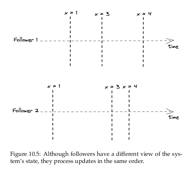
In the single machine/single-threaded case, the actions that we take are “seemingly” instaneous (after writing, the state change immediately).

In the case where the state is replicated, it is not the same. Let us assume that we have a multiple-node system that implement Raft leader election and Raft state machine replication. Write requests are then served by the leader only. Having read requests also served by the leader only seems unintuitive since it limits the system’s capability. If the read requests are served by followers, there can be the case where the follower does not have the latest data, and it leads to inconsistency.

Intuitively, there is a tradeoff between how consistent the observers’ views of the system are and the system’s performance and availability. To understand this relationship, we need to define precisely what we mean by consistency. We will do so with the help of consistency models, which formally define the possible views the observers can have of the system’s state.

10.3.1 Strong consistency

It is the model that is similar to the first diagram of the previous explanation that I gave. Another word for strong consistency is linearizability.

10.3.2 Sequential consistency

The consistency model that ensures operations occur in the same order for all observers, but doesn’t provide any real-time guarantee about when an operation’s side-effect becomes visible to them, is called sequential consistency. The lack of real-time guarantees is what differentiates sequential consistency from linearizability.

A producer / consumer system synchronized with a queue is an example of this model; a producer writes items to the queue, which a consumer reads. The producer and the consumer see the items in the same order, but the consumer lags behind the producer.

10.3.3 Eventual consistency

Although we managed to increase the read throughput, we had to pin clients to followers – if a follower becomes unavailable, the client loses access to the store. We could increase the availability by allowing the client to query any follower. But this comes at a steep price in terms of consistency. For example, say there are two followers, 1 and 2, where follower 2 lags behind follower 1. If a client queries follower 1 and then follower 2, it will see an earlier state, which can be very confusing. The only guarantee the client has is that eventually all followers will converge to the final state if writes to the system stop. This consistency model is called eventual consistency.

It’s challenging to build applications on top of an eventually consistent data store because the behavior is different from what we are used to when writing single-threaded applications. As a result, subtle bugs can creep up that are hard to debug and reproduce. Yet, in eventual consistency’s defense, not all applications require lineariability. For example, an eventually consistent store is perfectly fine if we want to keep track of the number of users visiting a website, since it doesn’t really matter if a read returns a number that is slightly out of date.

Notes

I cannot differentiate sequential consistency and eventual consistency. I feel like they might be something related to… state building. Suppose our state is a single number x. We also have operations ops to modify x.

If ops only consists of + operations, for example:

+1
+3
+2
+9

Then if we look at the final state, it doesn’t matter if +1 is applied before or after +9. In mathematics’s terminology, the operations are “associative”. The system can be “eventual consistency” here.

If ops consists of +, -, *, and / operations, for example:

+1
*3
/5
-9
*9

Then suddenly, the order matters. (x + 1) * 3 is different from (x * 3) + 1. “Sequential consistency” is needed.

10.3.4 The CAP theorem

When a network partition happens, parts of the system become disconnected from each other. For example, some clients might no longer be able to reach the leader. The system has two choices when this happens; it can either:

• remain available by allowing clients to query followers that are reachable, sacrificing strong consistency
• or guarantee strong consistency by failing reads that can’t reach the leader.

The concept is expressed by the CAP theorem, which can be summarized as: “strong consistency, availability, and partition tolerance: pick two out of three.” In reality, the choice really is on between consistency and availability, as network faults are a given an can’t be avoided.

[…]

I think this explanation from Wikipedia is more on-point:

• Consistency: every read receives the most recent write or an error
• Availability: every request receives a (non-error) response, without the guarantee that it contains the most recent write.
• Partition tolerance: the system continues to operate despite an arbitrary number of messages being dropped (or delayed) by the network between nodes

No distributed system is safe from network failures, thus network partitioning generally has to be tolerated. In the presence of a partition, one is then left with two options: consistency or availability.

• When choosing consistency over availability, the system will return an error or a time out if particular information cannot be guaranteed to be up to date due to network partitioning.
• When choosing availability over consistency, the system will always process the query and try to return the most recent available version of the information, even if it cannot guarantee it is up to date due to network partitioning.

Also, even though network partitions can happen, they are usually rare within a data center. But, even in the absence of a network partition, there is a tradeoff between consistency and latency (or performance). The stronger the consistency guarantee is, the higher the latency of individual operations must be. This relationship is expressed by the PACELC theorem, an extension to the CAP theorem. It states that:

• In the case of network partitioning (P), one has to choose between:
  • Availability (A) and
  • Consistency (C)
• But else (E), even when the system is running normally in the absence of partitions, one has to choose between:
  • Latency (L) and
  • Consistency (C)

In practice, the choice between latency and consistency is not binary but rather a spectrum.

This is why some off-the-shell distributed data stores come with counter-intuitive consistency guarantees in order to provide high availability and performance. Others have knobs that allow you to chooose whether you want better performance or stronger consistency guarantees […].

Another way to interpret the PACELC theorem is that there is a trade-off between the amount of coordination required and performance. One way to design around this fundamental limitation is to move coordination away from the critical path. For example, earlier we discussed that for a read to be strongly consistent, the leader has to contact a majority of followers. That coordination tax is paid for each read! In the next section, we will explore a different replication protocol that moves this cost away from the critical path.

10.4 Chain replication

[…]. In chain replication, processes are arranged in a chain. The leftmost process is referred to as the chain’s head, while the rightmost one is the chain’s tail.

Clients send writes exclusively to the head, which updates its local state and forwards the update to the next process in the chain. Similarly, that process updates its sate and forwards the chain to its successor until it eventually reaches the tail.

When the tail receives an update, it applies it locally and sends an acknowledgement to its predecessor to signal that the change has been committed. The acknowledgement flows back to the head, which can then reply to the client that the write succeeded.

Client reads are served exclusively by the tail […]. In the absence of failures, the protocol is strongly consistent as all writes and reads are processed one at a time by the tail. But what happens if a process in the chain fails?

Falut tolerance is delegated to a dedicated component, the configuration manager or control plane. At a high level, the control plane monitors the chain’s health, and when it detects a faulty process, it removes it from the chain. The control plane ensures that there is a single view of the chain’s topology that every process agrees with. For this to work, the control plane needs to be fault-tolerant, which requires state machine replication (e.g., Raft). So while the chain can tolerate up to N - 1 processes failing, where N is the chain’s length, the control plane can only tolerate C / 2 failures, where C is the number of replicas that make up the control plane.

There are three failure modes in chain replication:

• The head can fail,
• The tail can fail, or
• An intermediate process can fail.

If the head fails, the control plane removes it by reconfiguring its successor to be the new head and notifying clients of the change. If the head committed a write to its local state but crashed before forwarding it downstream, no harm is done. Since the write didn’t reach the tail, the client that issued it hasn’t received an acknowledgement for it yet. From the client’s perspective, it’s just a request that timed out and needs to be retried. Similarly, no other client will have seen the write’s side effects since it never reached the tail.

If the tail fails, the control plane removes it and makes its predecessor the chain’s new tail. Because all updates that the tail has received must necessarily have been received by the predecessor as well, everything works as expected.

If an intermediate process X fails, the control plane has to link X’s predecessor with X’s successor. This case is a bit trickier to handle since X might have applied some updates locally but failed before forwarding them to its successor. Therefore, X’s successor needs to communicate to the control plane the sequence number of the last committed update it has seen, which is then passed to X’s predecessor to send the missing updates downstream.

Chain replication can tolerate up to N - 1 failures. So, as more processes in the chain fail, it can tolerate fewer failures. This is why it’s important to replace a failing process with a new one. This can be accomplished by making the new process the tail of the chain after syncing it with its predecessor.

The beauty of chain replication is that there are only a handful of simple failure modes to consider. That’s because for a write to commit, it needs to reach the tail, and consequently, it must have been processed by every process in the chain. This is very different from a quorum-based replication protocol like Raft, where only a subset of replicas may have seen a committed write.

Chain replication is simpelr to understand and more performant than leader-based replication since the leader’s job of serving client requests is split among the head and the tail. The head sequences writes by updating its local state and forwarding updates to its successor. Reads, however, are served by the tail, and are interleaved with updates received from its predecessor. Unlike Raft, a read request from a client can be served immediately from the tail’s local state without contacting the other replicas first, which allows for higher throughput and lower response times.

However, there is a price to pay in terms of write latency. Since an update needs to go through all the processes in the chain before it can be considered committed, a single slow replica can slow down all writes. In contrast, in Raft, the leader only has to wait for a majority of processes to reply and therefore is more resilient to transient degradations. Additionally, if a process isn’t available, chain replication can’t commit writes until the control plance detects the problem and takes the failing process out of the chain. In Raft instead, a single process failing doesn’t stop writes from being committed since only a quorum of processes is needed to make progress.

That said, chain replication allows write requests to be pipelined, which can significantly improve throughput. Moreover, read throughput can be further increased by distributing reads across replicas while still guaranteeing linearizability. […]

You might be wondering at this point whether it’s possible to replicate data without needing consensus at all to improve performance further. In the next chapter, we will try to do just that.

So in short, from the author’s comparison Raft has better write throughput and might have lower read throughput than chain replication.

Chapter 11 Coordination avoidance